
By Guillaume Matheron, Johan Sassi, Alexander Belikov
At Hello Watt we help consumers reduce their bills by comparing energy providers. We offer a web platform that lets consumers monitor and analyze their energy consumption over time, and a set of tools for planning home renovations.
While our goal is to accompany consumers in their energy transformation journey or everyday life energy consumption, acquisition of new users is critical to our growth strategy which is why we employ both SEO (Search Engine Optimization) and SEA (Search Engine Advertising) marketing strategies. SEA marketing consists of posting advertisements on the results page of search engines. We predominantly use the Google search engine for that purpose and are always trying to improve the way we bid to optimize our budget.
In this article, we give a brief overview of the Google Ads platform from the point of view of an advertiser as well as its available performance indicators and controls. We show how a simple portfolio optimization method indicates we can increase our ad returns significantly. Finally, we design a more complex model that takes into account market saturation and show that the actual portfolio optimized by Google is very close to the maximum possible return predicted by our model.
Inner workings of Google Ads
Google provides an online console to manage ads and budgets. Each advertiser can manage several campaigns, that are split in “Ad Groups” each containing a set of “keywords”. On each Google search results page, a fixed number of slots are dedicated to ads. Each time there is a search request, Google executes an automatic auction between all advertisers that have made bids for keywords matching the search query.
From the point of view of an advertiser, two modes are available to handle a campaign: the automatic mode lets Google engine set bids automatically, while in the manual mode the advertiser can set a maximum bid for each ad group.
Both the auction process itself and the automatic bid selection algorithm behave like black boxes and are not well documented. However, we can hypothesize the auction to behave as a Vickrey auction in which the highest bid wins the ad slot, but at the price given by the second-best offer.
Outline
In this article, we attempt to formulate an optimization problem that maximizes the return of ad campaigns by controlling the bidding process and budgets.
First, we describe metrics that can be used as proxies for the performance of a campaign, then we formulate a market model that takes into consideration our investment in each keyword or ad group. Finally, we show that this model can be used to solve a global non-convex optimization problem that yields a budget allocation strategy maximizing the expected return for a given target volatility and total budget.
Performance indicators
The performance of a SEA campaign can be described by several metrics, each of which can be calculated with a varying degree of certainty. For instance, the number of impressions or clicks is readily available, however metrics based on value, which are directly related to monetary performance require downstream information about acquisitions. Since, for example, the attribution of acquisitions to a source (be it a particular ad or natural search) involves unobserved steps, performance-based metrics are less certain.
Clicks, acquisitions and various derived metrics may be strongly correlated with many factors that can be observed (search terms, time of day), measured (number of visits) or inferred (gender, age group, income range).
For instance, there is subpage on the Hello Watt website that reports the real-time cost of electricity on the following day (some providers have variable rates). Users who enter search terms containing “tomorrow” are most likely interested in browsing this page for which the conversion rate is very low, however users who enter other queries are more likely to be interested in our high-value services.
While the total ad campaign value is of interest, more often than not relative indicators such as value-per-click (VPC) or value-per-impression (VPI) may be used as indicators.
On the other hand, the cost of the campaign over a period of time or a portion of the audience is also monitored, since the investment may be allocated unevenly, both over time and over portions of the audience to optimize costs.
The ratio of value over cost is expressed as Return Over Advertising Spend (ROAS), and is the quantity we attempt to optimize.
Markowitz strategy
It is a common practice to split visitors in segments depending on their age group, gender, the time of day or and any other factor that can be observed, measured or inferred. The caveat is that the finer the segmentation, the fewer data points are available in each segment which decreases the statistical significance of performance indicators. Therefore, it is important to choose a pertinent and parsimonious segmentation.
Once a segmentation is chosen, a reasonable question is how to split the advertising budget between these categories. For instance, it seems logical to spend more on people who are more likely to buy our services, whether that means making higher bids or bidding more often on their search queries. In a sense we are splitting our budget among assets which have different expected returns. This formulation leads to a natural parallel with monetary portfolio optimization where assets are segments, and the expected return of an asset is the ROAS for this segment.
If the ROAS were deterministic, an obvious solution would be to spend all our ad budget on a single segment. However, we observe the variations of ROAS week over week and thus can compute its variance over time, which is a proxy for the risk of investing in this segment. This is direct analogy to the portfolio optimization model where the risk of an asset is measured in terms of volatility.
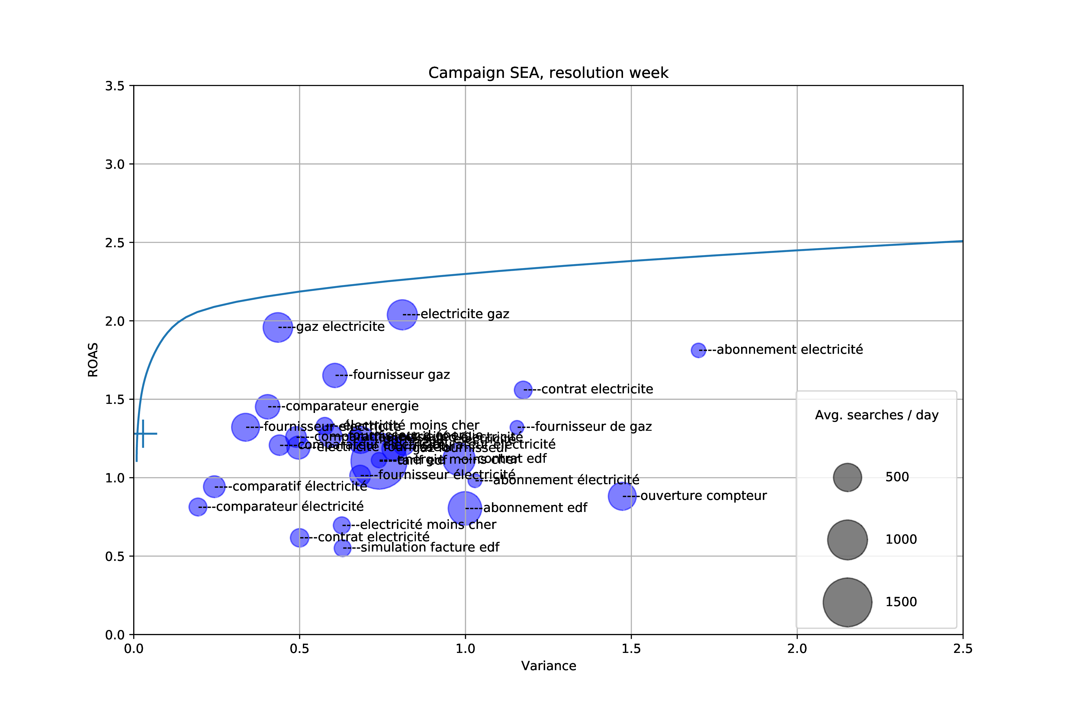
In the figure below, we split our visitors depending on the keywords in their search query, and plot them according to their average ROAS and measured variance of ROAS week over week. The size of each bubble is the number of search queries that occur in each segment.

For instance, the most profitable keyword combination is “gaz électricité” with an average return of 2.0. However, the most stable keyword over time is “comparateur électricité” even though its ROAS is less than 1.
Given the list of assets, their profitability and risk, a portfolio has itself an expected return and variance, which can be plotted on the same diagram. A Markowitz model formulation allows us to compute the “efficient frontier” which represents the boundary of all possible portfolios. Any portfolio below the efficiency frontier could be made either more profitable for the same risk, or less risky for the same profits. Therefore, an optimal portfolio can be identified by a point on the efficient frontier which represents a risk/benefit trade-off (note that the full Markowitz theory handles covariances which we did not take into account in our experiments).
In the figure above the efficient frontier is plotted as a blue line, and the current ROAS and variance of our campaign is plotted as a large cross on the left side.
It appears that our campaign portfolio is very close to the efficient frontier of possible portfolios given the segments. It has a much lower variance than any single keyword combination, while having a higher return than most.
However, this graph suggests we can increase the return by 50% while maintaining a small variance. Trying to exploit this finding reveals the main issue of the Markowitz model as applied to our problem: it assumes there exists an infinite supply of each asset, which is not the case in our market.
Market saturation model
An intuitive view of market saturation is that if a commodity such as search queries are in limited supply, then increasing our spending will have diminishing returns. In the limit, spending an infinite amount will at most buy the full available supply.
Single Asset Model
We start with a simple model and assume that the searches budget for each segment is divided proportionally to the expenses of each competitor.
That is, if there are n competitors that have budgets cᵢ for i = 1..n, and there are s searches for a given period, then each competitor will get s × cᵢ/(∑ c ᵢ) ad impressions.
When looking at the data from the perspective of one of the competitors (ourselves), we rather define c as our own budget, and cc as the budget of all other competitors. We also define H as the expected return value per impression.
Our market model is therefore able to express the expected total return v given a budget c:
\(v = H s \frac{c}{cc + c}\)
As expected when our budget c is small the return v is a linear function, but when c goes to infinity, due to diminishing returns per impression the total return never exceeds H × s.
Portfolio model
When applying this model to a portfolio of assets that have different budgets cᵢ, competitors budgets ccᵢ, values per impression Hᵢ and number of searches per time period sᵢ, the expected value and variance of the portfolio can be computed as :
\( E[V] = \sum_i E[H_i s_i] \frac{c_i}{\textrm{cc}_i+c_i} \)
\( \textrm{Var}[V] = \sum_i \textrm{Var}[H_i s_i] \frac{c_i}{\textrm{cc}_i+c_i} \)
The values of E[Hᵢ sᵢ] and Var[Hᵢ sᵢ] can be either measured directly or inferred from historical data. Similarly, the budget of our competitors cc can either be inferred or computed using the existing metrics. In our case we used the reported impression share from Google Ads data to get an estimate of cc through our market model.
Optimization procedure
The objective of our portfolio allocation strategy is to maximize the expected revenue E[V] while minimizing variance Var[V]. Multi-objective optimization problems typically have several solutions that form the Pareto-efficient boundary. In our case, we want to output a set of portfolios such that their return cannot be increased without also increasing their variance.
Since we want to output several solutions and decide manually the best one based on a graphical representation, we use an a posteriori method. We to iterate over a sequence of possible value for E[V], then run a single-objective optimization algorithm to minimize Var[V] under the constraint of a target E[V]. By repeating this process, we generate a sequence of portfolio that are Pareto-efficient: E[V] cannot be increased without also increasing Var[V].
The single-objective optimization process itself is non-convex, and we tackle it using the L-BFGS-B algorithm.
Global non-convex optimization solution
The L-BFGS-B implementation we used (scipy.optimize) does not support explicit constraints, therefore they were introduced as negative loss terms.
This is the loss we used for a given portfolio in the form of a list of cᵢ:
\( L = Var[V] + 10^3 (E[V] – \textrm{target_return})^2 + 10^4 (c – \textrm{target_total_budget})^2 \)
The weight constants were chosen by monitoring the value of the constraints on the output plots of the optimization and applying trial-and-error to keep the errors under an acceptable bound for the full range of E[V] target values.
Results
By running this minimization problem several times with variable target returns, we can compute optimal portfolios for all achievable target returns.
Since multiple solutions exist in many cases, while scanning target returns in increasing order we use each solution as the initial guess of the next optimization problem. This helps stabilize the solutions and produces an output which is more readable.
The following plots show a series of stacked bars where each column represents a portfolio that minimizes variance (not displayed) for a given expected return in euros per week (x-axis). The black vertical bar shows the current return achieved by our campaign, while the right-hand stack plot shows the current portfolio at our company. The y-axis is in euros per week, and all simulated portfolios represent the same budget, but with different allocations among segments. Therefore, the right-hand side of the figure depicts portfolios that have greater ROAS at the cost of greater variance of returns.
Plot using ad group segmentation:
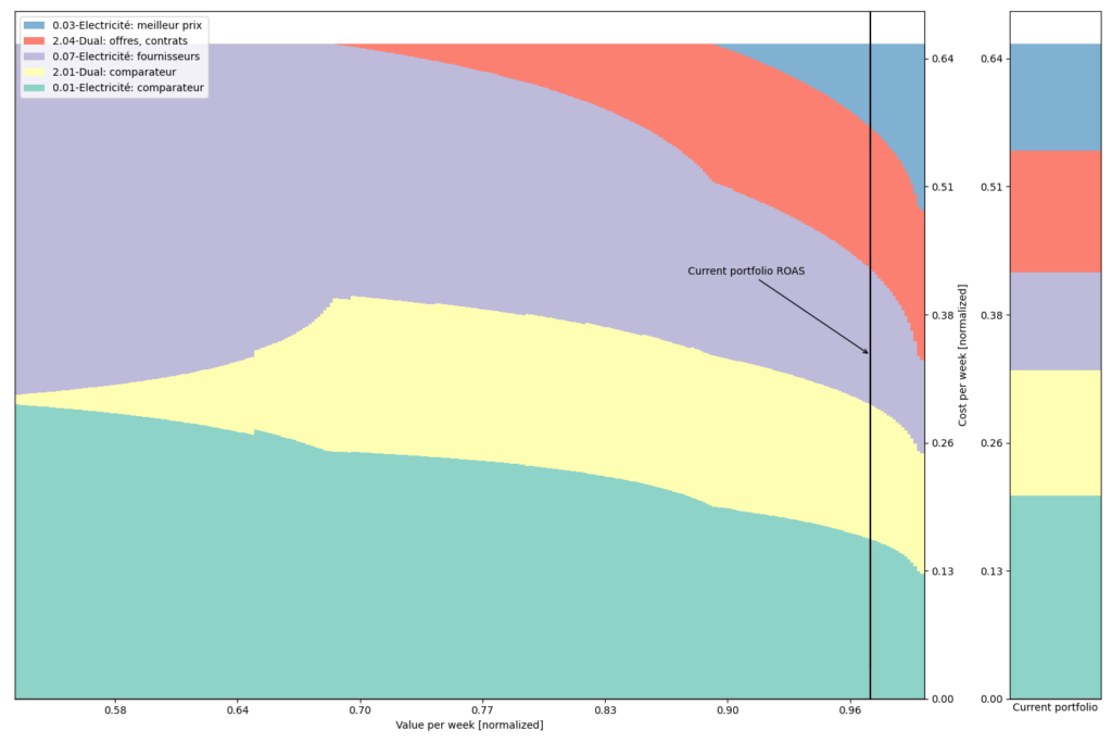
When targeting a low ROAS, the safest option is to invest in only two ad groups that are “Électricité fournisseurs” and “Électricité comparateur”. However, as we introduce new ad groups such as “Dual comparateur” then “Dual offres, contrats” and finally “Électricité meilleur prix”, we increase our gains at the cost of greater variance.
One interpretation is that “Électricité meilleur prix” is more valuable and at the same time less stable ad group, which should only be utilized for high-risk, high-reward spending strategies.
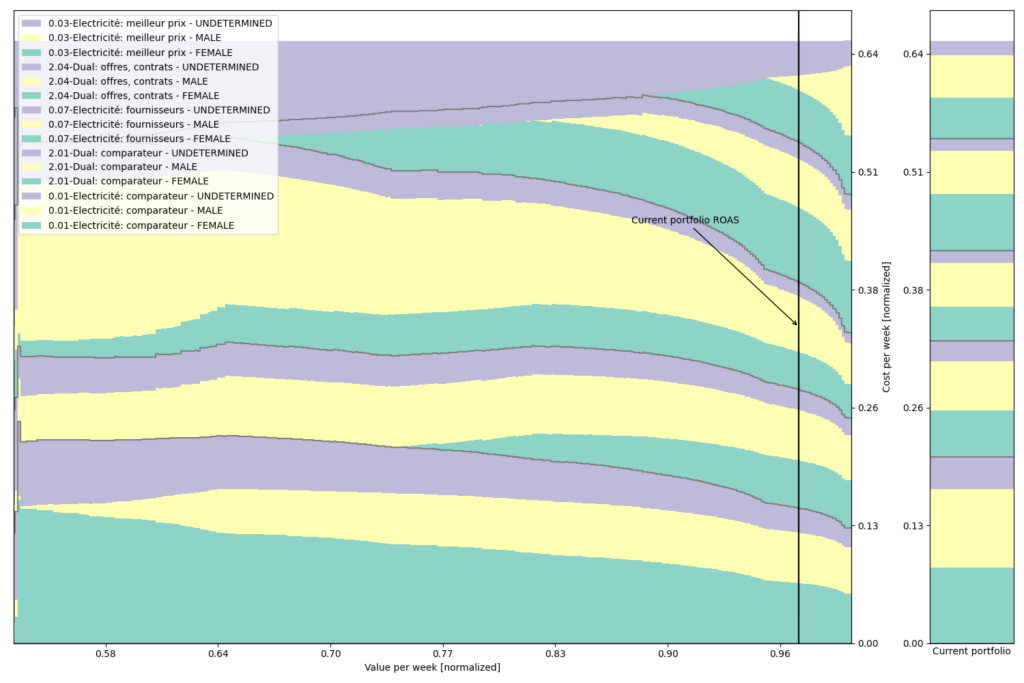
We reproduce this graph with finer segmentation, including gender stratification:
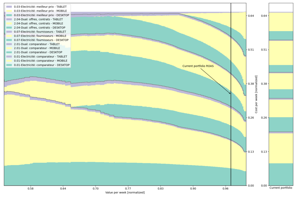
or device type:
Limitations
Our market saturation model take into account neither covariance (interaction between segments) nor is it designed to handle temporal trends. It uses variance of ROAS evaluated over weekly periods as a proxy for volatility, which may be subject to bias and variance.
Moreover, our model assumes not only that our changes in ad spending will not affect the behavior of our competitors, but also that their behavior does not vary during the analyzed period. To justify this assumption we restricted the study to three months, which represents a compromise between the statistical significance and the temporal consistency of the observed behavior.
Yet another assumptions we make is related to a simplified view of the Google’s black box bidding process: we assume the available ad slots on search queries are distributed according to budget. In addition to that we assume that the cost of ads within a single segment is near-constant.
Conclusion
A simple portfolio optimization strategy we used initially suggested we could greatly improve our returns. However, a more sophisticated model that takes into account market saturation effect indicates that the current portfolio (optimized by the Google engine) is very close to the maximum possible return regardless of variance. The observed portfolio itself occasionally deviates from the predicted by the model, but the differences are not important enough to warrant manual action on the budgets. This seems to indicate that Google’s internal bidding algorithm is already optimizing for these metrics, in a way that seems fair to the advertisers given the available data and our hypotheses.