Published in Energy and Buildings, PDF version on arxiv
Authors: Guillaume Matheron, Johan Sassi, Alexander Belikov
In this article we present an unsupervised low-frequency method aimed at detecting and disaggregating the power used by Cumulative Water Heaters (CWH) in residential homes. Our model circumvents the inherent difficulty of unsupervised signal disaggregation by using both the shape of a power spike and its temporal pattern to identify the contribution of CWH reliably. Indeed, many CHWs in France are configured to turn on automatically during off-peak hours only, and we are able to use this domain knowledge to aid peak identification despite the low sampling frequency.
In order to test our model, we equipped a home with sensors to record the ground truth consumption of a water heater. We then apply the model to a larger dataset of energy consumption of Hello Watt users consisting of one month of consumption data for 5k homes at 30-minute resolution. In this dataset we successfully identified CWHs in 66.5% of cases where consumers declared using them. Inability of our model to identify CWHs in the consumption signal in the remaining cases is likely due to possible misconfiguration of CWHs, since triggering them during off-peak hours requires specific wiring in the electrical panel of the house. Our model, despite its simplicity, offers promising applications: detection of mis-configured CWHs on off-peak contracts and slow performance degradation.
1. Introduction
Smart meters in France. In an effort to record and optimize energy consumption of households as well as facilitate billing, starting from the beginning of
century multiple countries around the world, including France, developed programs aiming at mass deployment of smart meters [1, 2]. By the end of 2021 about 34 million smart meters, called Linky, were installed in France [3].
Signal disaggregation. Linky records energy consumption data at intervals of 30 minutes (or in a small number of cases 10 minutes) and uploads it to the data storage infrastructure of Enedis, the French energy distribution company, through power-line communication [4], while technical and contractual data is retrieved from energy providers. Since the characteristic operational time scales of most appliances are in the order of minutes, disaggregation of the total signal is a difficult task.
There exist a number of publicly available ground truth datasets, see for example [5, 6, 7]. Each dataset is country-specific and therefore provides a typical sample of a country-specific distribution of appliances per household, thus hindering the application of supervised disaggregation methods for underrepresented appliances. In France a variety of options are available to residential consumers for heating water, with most popular modes being cumulative water heaters (CWH), gas heaters and collective heating. To our knowledge there are no publicly available large-scale ground truth datasets for cumulative water heaters.
CWHs as targets for disaggregation. Cumulative Water Heaters are good targets for disaggregation due to the following reasons:
- In the residential sector in France, water heating is one of the main contributors to energy consumption (about 12%, second to heating that accounts for 61% of consumption [8]).
- Its average ”ON” time is typically greater than the time resolution of low frequency meters, such as Linky. Typical volume is in the range of 40 to 300 litres, and the average time required to heat a full load of water to operational temperature varies between 1.5 and 5 hours depending on volume and power [9].
- Most electrical energy providers for residential consumers in France offer contracts with split pricing, where the price of energy is about 25 to 30% cheaper during off-peak hours. In this article, we use the term HP/HC (from French “Heures Pleines / Heures Creuses”) when referring to split pricing, and “off-peak hours” when referring to the period during which electricity is cheaper. HP/HC is one of examples of dynamic pricing that also include the so-called EJP [10], (from French “Effacement Jour de Pointe”, translated as “Peak shaving day”) and TEMPO [11]. The former offers a reduced price of energy for 343 days a year and a much increased price of energy for selected remaining 22 days. The latter offers three types of color-coded days with HP/HC, i.e. a grid of tarifs changing from 0.0862€ for offpeak hours during blue days to 0.5486€ for peak hours during red days (EDF data for March 2022). The HP/HC hours are reported from the energy provider to the meter through power-line communication. Then users have an option to synchronize their use of appliances with off-peak hours, which can be achieved automatically, either via a timer or a signal from a pilot wire connected to a device that detects the activation of off-peak hours using a signal sent through the electrical mains [12].
We therefore expect a CWH, correctly connected to the pilot wire, to reliably switch on at the beginning of each off-peak interval and remain in that state until the full tank is heated to its target temperature. Under normal usage each “ON” cycle lasts more than 30 minutes which is the time resolution of Linky data [9].
Hello Watt is an energy consulting firm for residential consumers, that also provides monitoring and analysis services.
Residential consumers may opt-in to share their energy consumption data and some of their metadata such as the type of water heating, through a consent form signed per household as mandated by French and European laws. The insights drawn from the analysis of large representative data samples helps to solve real-world user problems, reduce energy consumption and bills, improve the quality of life. In this paper we present a novel disaggregation method for CWHs in Section 3 and study its performance on a labeled dataset in Section 4. In Section 5 we present a large anonymized sub-sample of Hello Watt user consumption data (about 5k users) (and make it publicly available) and in Section 6 the results of application of our CWH model to this dataset. We conclude with a brief discussion in Section 7.
2. Related Work
Disaggregation of energy consumption curves is a main component of Non-Intrusive Load Monitoring (NILM), which is an active research area.
When the aggregated load curve is available at a high time resolution, many approaches are possible such as event matching, where device activation edges are identified and matched to appliances [13] and feature recognition [14]. Deep learning has also been used to successfully disaggregate load curves using training data [15, 16, 17, 18]. These approaches use deep recurrent neural networks such as Long Short-Term Memory, but some solutions also exist that use only feed-forward networks [19, 20, 21]. Other approaches model the consumption behavior of a building as a Hidden Markov Model, where combinations of device activations are modeled as states of a Markov chain which is partially observed [22]. The last approach is especially relevant in our case because it has been successfully applied to sampling rates as low as one sample per minute.
However, our use case requires algorithms that can process even lower sampling rates, down to one sample per 30 minutes. At this resolution, most approaches are device-specific. For instance, authors of [23] use the statistical relationship between daily energy consumption and exterior temperature to disaggregate the electrical heating component.
3. Disaggregation Method for Devices with Regular Time Signatures
Our disaggregation method is based on the observation that CWH consumption signal has regular features: time signature of activations linked to beginning of off-peak hours and sufficiently long active periods. The method consists of two parts. First, we compute the threshold for background consumption and tag data points that exceed this threshold as candidate spikes (spike detection). In the second step we identify whether there exists a pattern of spikes that matches the expected characteristics of the device of interest (spike filtering).
The input of our model is composed of an evenly spaced times series representing average power consumption, a set of monotonic intervals describing off-peak hour ranges \(\{(t^{(k)}_a, t^{(k)}_b)\}\), where \( 0 \le t^{(k)}_a < t^{(k)}_b < 24\), and a range for the expected power level of the device of interest.
The output of our model is a list of activation times, durations and power usage of the device of interest.
In this publication electrical power is expressed in kW units. Time series are given with a frequency of 30 minutes, and off-peak range boundaries are rounded to 30-minute increments.
Spike detection. The first step of our pipeline is to compute the background noise threshold, identify spikes that exceed it and store whether their start coincides with the start of off-peak hours.
- We split the time series into a list of smaller sections that are handled independently (in our application we split the input into 7-day segments). These sections are later referred to as observations. This step reduces the sensitivity of downstream steps to the amount of input data, and handles consumption drift.
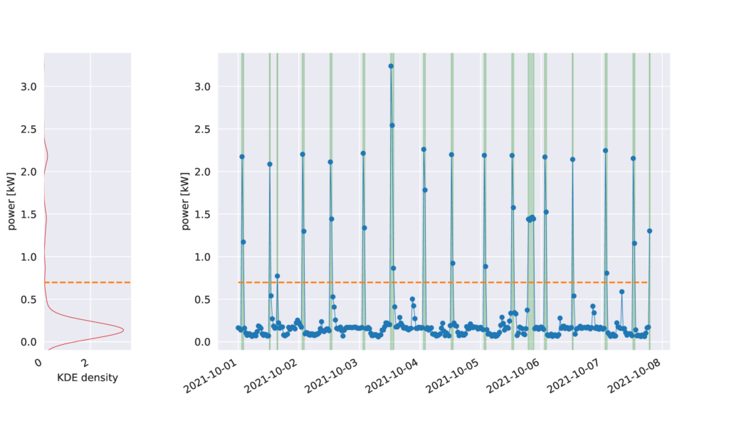
- We apply a Kernel Density Estimator (KDE) to each observation independently, and use the first local minimum of the estimator as the threshold between background and spike consumption2 . We use Scott’s rule to select the KDE bandwidth [24] (this process is depicted in Figure 1, where the red curve in the left subplot represents the KDE).
- For each observation, we select sequences of consecutive consumption values that are above the threshold. These are referred to as spikes. For each spike we store the start time of the spike relative to the closest start of off-peak hours as well as the maximum power used during the spike, minus the local background power level. In this last step, we estimate the background power level as the average of two closest data points that are outside the spike. Indeed, as can be seen in Figure 1, the computed threshold is well above the background level and only serves as a classification boundary.
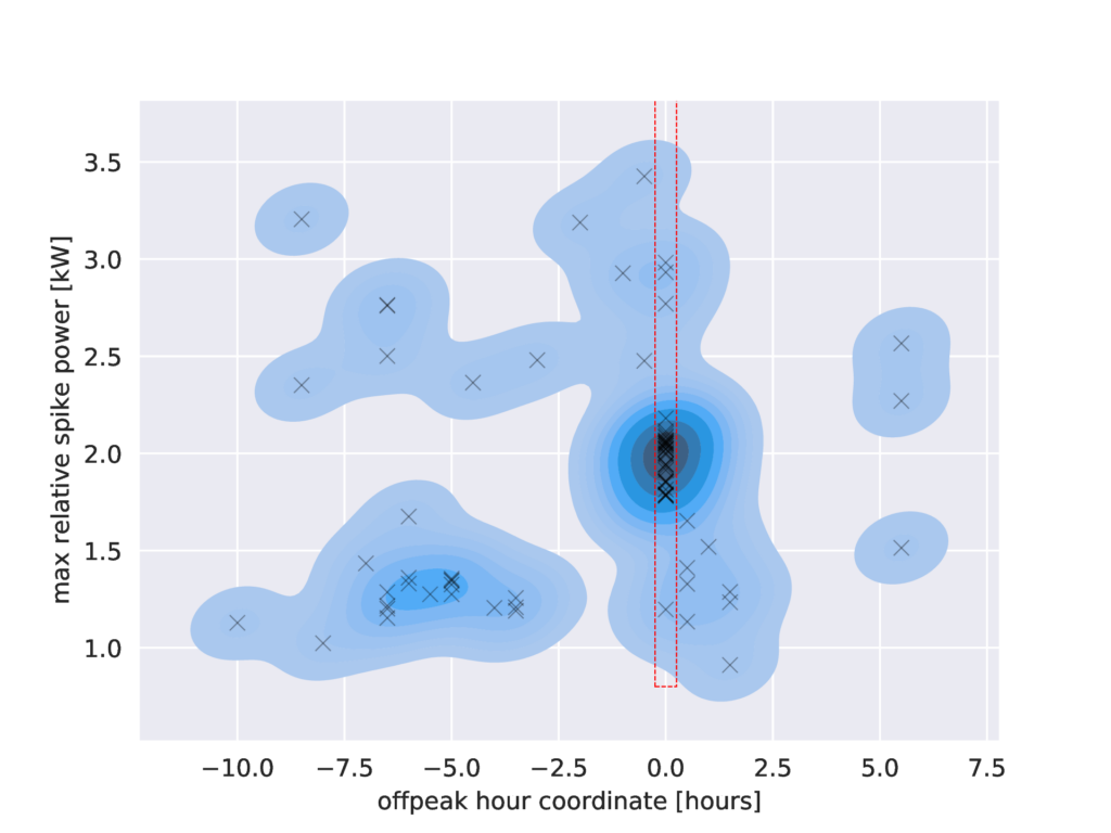
Spike filtering. Figure 2 shows a density plot of the characteristics of the spikes identified in the previous step. The filtering step of the algorithm identifies whether a cluster matching the expected characteristics of a CWH exists in this space.
Two conditions must be met for a spike to be classified as being caused by a CWH: (a) it starts exactly at the beginning of off-peak hours (this is represented as a red box in Figure 2); (b) the set of all spike power levels that validate criteria (a) form a cluster within the expected range for the target device (in our case 0.8 to 5 kW).
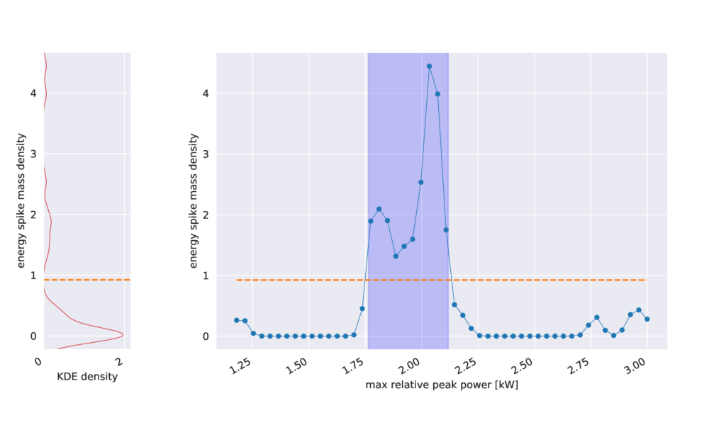
The clustering step in (b) uses KDE again to find a spike in the space of power levels, much like the spike identification step uses KDE to find spikes in time. The second clustering step is depicted in Figure 3.
If the identified spike matches the expected power of the device of interest, then the fit is considered successful and all matching power spikes can be attributed to this device.
4. Model Validation
In order to validate our model, we equipped a single home with a custom electric meter that provided a ground truth by measuring the power of the CWH about once per second. These power readings were aggregated into a measure of energy consumption at a resolution of 30 minutes to match the measures collected by the energy provider. In parallel, the overall consumption of this home is independently reported through its smart meter and collected from the energy provider at a resolution of 30 minutes.
This experiment was conducted during 47 days, mostly in February 2022.
Therefore, we were able to test the disaggregation model against a known baseline. Figure 4 shows the load curve of the home during the testing period, and colors are superimposed to show over and under-estimations of the water heater consumption according to our model.
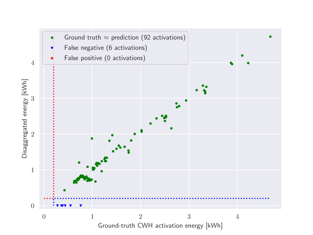
Figure 5 shows activations of the water heater (an activation being defined as a series of consecutive 30-minute intervals where the average power of the CWH is greater than 400 watts). It demonstrates that most of the activations of the water heater were properly detected, the only exceptions being very short activations that occur early in the morning when the water heater re-activates before the end of the off-peak period (for instance when someone takes an early shower). No false positives were identified in terms of activations (all detected activations correspond to a ground-truth one), meaning that when viewed as a test for activations of the CWH, our model has a precision of 100 %. The false negatives amount to a recall of 93.9 % .
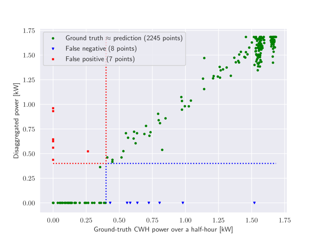
In a complementary way, Figure 6 shows each individual 30-minute period, and we can see both some false positives where CWH consumption was wrongly identified, and some false negatives where an interval was wrongly identified as not being part of a CWH activation.
For a given 30-minute interval, we use our model to detect whether the CWH used more than 400 watts on average. The statistics of this test are presented in Table 1.
However, these over and under-estimations happen mostly at the trailing edge of CWH activations: the activation itself is recognized with high accuracy, but its predicted duration is not always exact, especially when it ends early in the last half-hour period. In these cases the last 30-minute interval blends into the background and is hard to identify, however this has little effect on the computed energy of the activation as a whole which is why we picked 400 watts as the threshold for a meaningful contribution of the CWH4 .
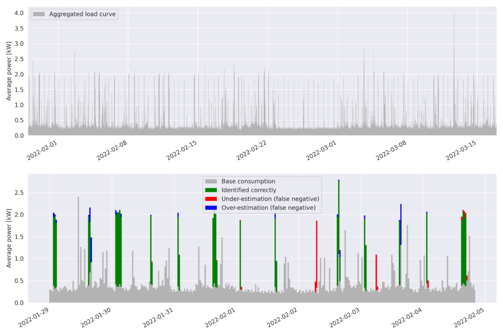
Bottom: First 7 days of the same load curve. For each 30-minute interval, the portion of consumption that was identified correctly as CWH is green, the portion that was identified correctly as non-CWH is grey, portions that were mistakenly identified as CWH are blue and portions that were mistakenly identified as non-CWH are red.
Concretely, for a given 30-minute interval, let \(t\) be the total consumption as reported by the meter, \(g\) be the ground-truth CWH consumption, \(m\) be the CWH consumption according to the model. A grey bar of height \(t-g\) is displayed, then a green bar of height \(min(m, g)\). Finally if \(g>m\) then a red bar of height \(g-m\) is stacked, otherwise a blue bar of height \(m-g\).
| True positives | 195 |
| True negatives | 2050 |
| False positives | 7 |
| False negatives | 8 |
| Precision | 96.5 % |
| Recall | 96.1 % |
5. Hello Watt Dataset Description
Hello Watt collects power usage data at a resolution of 30 minutes. Among all Hello Watt users, approximately 46% have HP/HC pricing. Among Hello Watt users who declared using a CWH, 66% have HP/HC pricing. We expect a higher proportion of HP/HC contracts in the CWH user group compared to the overall sample because HP/HC pricing is financially beneficial for households with loads that can easily be scheduled, such as CWHs. The distribution of water heating types, and the fraction of contracts with HP/HC pricing is presented in Table 2.
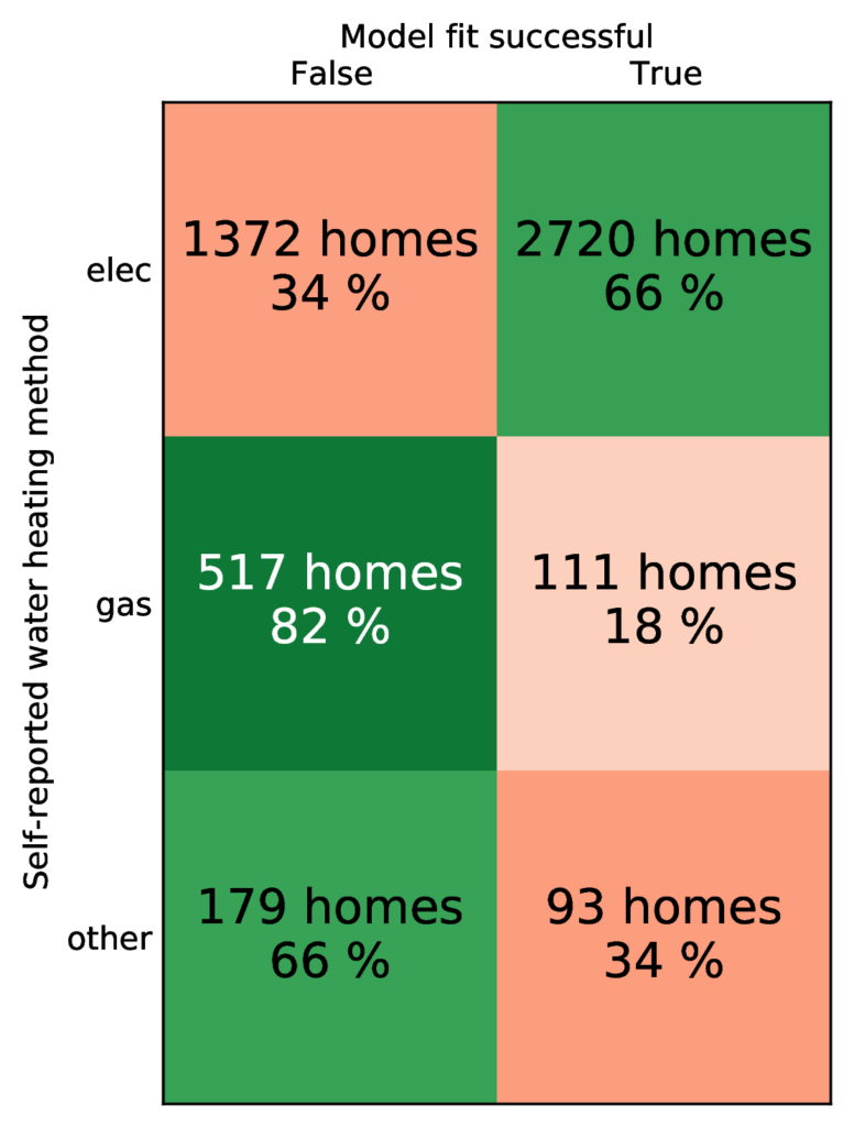
To develop and test our disaggregation method we consider a subsample consisting of power consumption of 5k households with HP/HC pricing contracts for one month. The number of households per water heating type in this dataset is presented in Figure 8. This dataset is published through the Open Science Framework5 . We chose to include in our dataset both homes with and without electric water heaters to validate the results of the model as presented in Section 4.
In addition to the type of their water heating, some users also provide such metadata as the home surface area, and the number of inhabitants.
Our working subsample consists of electricity consumers interested in their energy consumption, and therefore it may have some have a distributional bias.
| HP/HC | base | HP/HC frac. | Total | |
| elec | 15667 | 8238 | 66 % | 23905 (57 %) |
| gas | 2088 | 11609 | 15 % | 13697 (33 %) |
| other | 1119 | 3028 | 27 % | 4147 (10 %) |
| Total | 18874 | 22875 | 45 % | 41749 |
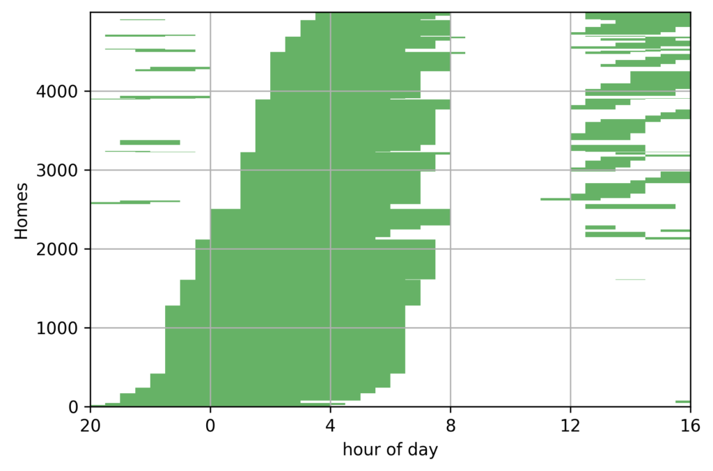
HP/HC contracts. For a given house and day, off-peak hours are made of up to three intervals, whose total duration is exactly eight hours. These times are always expressed in local time (timezone Europe/Paris) and for a given house they are usually identical for all days. The distribution of off-peak ranges in our sub-sample is presented in Figure 7. The off-peak hours are split in two intervals in 92% of houses, one continuous interval for 4% of houses, and three intervals for the remaining 4%.
6. Analysis of Hello Watt Dataset
In this section, we run the model on consumption data from October 2021, taken from a subset of houses from our database. These consist of a random sample of houses that meet the following criteria:
- Have at least 1440 (\(48\times 30\)) energy measure datapoints during the month of October 2021 (since October has 31 days, this allows for up to 3% of missing data, which can happen due to meter malfunctions).
- The technical and contractual data we retrieve from the energy provider indicates that the user has subscribed to an HP/HC contract.
- The off-peak hours are known for this house.
Each home can have one or several off-peak hour ranges, either during the night or the afternoon. Figure 7 shows all the off-peak ranges of the houses in the dataset. For each home, we also have self-reported data about the main mode of water heating, surface and number of inhabitants. Figure 8 shows self-reported water heating modes in the dataset.
These metadata allow us to test the ability of our model to distinguish homes with and without CWH by comparing its output with self-reported data.
6.1. CWH Detection
Since gas is easier to store than electricity, there is no equivalent to HP/HC for gas and the disaggregation method presented in this article does not apply. However, for verification we can still run our model on homes that have known off-peak hours for electricity but no electric water heater (gas, collective or no water heating at all). In that case we expect not to detect any electric water heater.
Results presented in Figure 8 reveal that in 66.5% of cases where the user has declared having an electric water heating we detect a device with on/off cycles compatible with off-peak hour triggering hypothesis. In cases when users declared using gas water heaters this fraction drops to 17.7 % .
The difference between self-reported metadata and model results can be attributed to (a) misreporting by users of water heating type, (b) incorrectly connected electric water heaters, (c) discrepancies between real off-peak hours and those available to us, and (d) users that match all the above conditions except that they have not resided in the home of interest during the observation period.
Indeed, some users may not know their type of water heating or purposefully report it erroneously, or they might have several types of water heating and forced to choose only one of them to report, since the registration form has only one field of entry. Some users may have HP/HC contracts but water heaters that trigger independently of off-peak hours because specific synchronization equipment was either not installed or mis-configured. It is likely that the explanation of high fraction of homes with reported CWH but negative model fit involves several factors.
To validate our conclusions about a relatively high value of unsuccessful fits for user-declared water heaters we ran an internal survey. Out of 32 participants, 8 reported having both electric water heaters and HP/HC contracts. Our model identified water heaters in 6 out of 8 cases. In both cases where no CWH was identified, visual inspection of the load curve revealed that a CWH is indeed present but did not turn on automatically at the start of off-peak hours (which was confirmed by users), supporting our hypothesis that a significant number of CWHs trigger independently of off-peak hours, and are not able to be identified by our model.
On the other hand false positives (successful model fits for types of water heating different from electric) may also be explained by other types of devices activated regularly during off-peak hours, such washing machines or dishwashers.
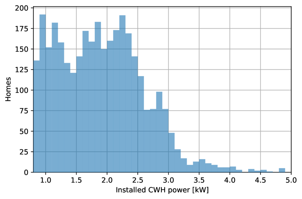
In Figure 9 we show the distribution of power levels of identified devices. Power levels of single-home residential water heaters offered by manufacturers form a discrete set starting from 0.8 W to 3 kW with a step 0.1 kW, but occasionally 0.2 or 0.05 kW. Therefore, we were motivated to use KDE with bandwidth of 0.1 kW and identified peaks at levels 1.1, 1.8, 2.2, 2.8, 3.5, 4.5 and 4.9 kW . While qualitatively the peaks we obtained are in agreement with domain knowledge (according to our observation most popular water heaters in the market have powers 1.2, 1.5, 1.6, 1.8, 2.2 kW etc), the accuracy of our current model does not allow us to separate peaks corresponding to different power-levels to adequate precision. Partially this might be due to a systematic effect related to the limits of water heater calibration, partially due to shortcomings of our model, which is based on simplified assumptions of deterministic noise, constant during the activation period of the water heater.
6.2. CWH Disaggregation Results
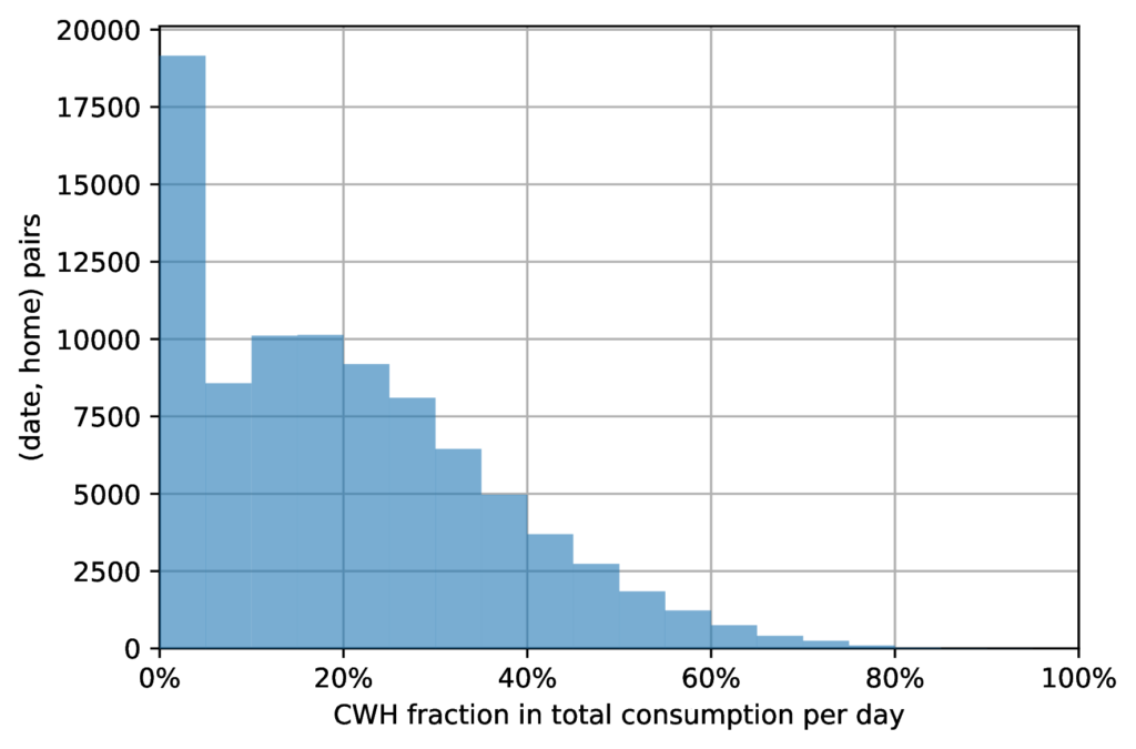
In Figure 10 we present the distribution of daily CWH consumption fraction. Each bar represents the number of days that correspond to CWH consumption within the bin’s bounds. The total number of days is about 88K, in accordance with the number of household where our model detected a functioning CWH. The spike at zero in the distribution of daily average corresponds to days when there was no hot water usage. While it is possible that tenants are away a fraction of time, we also note that our current model does not discover all the relevant peaks, especially if there are variations in background values.
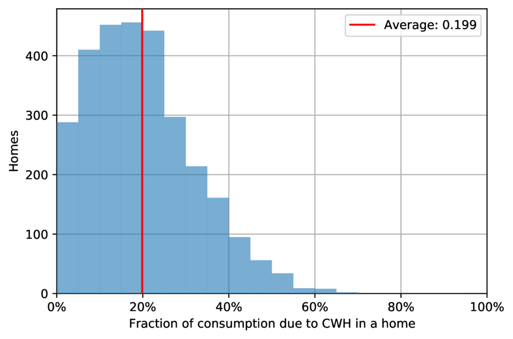
In Figure 11 for each household in our dataset we present the estimation of the total consumption fraction due to identified CWHs over the observation period. The distribution of the total consumption fraction due to CWH is unimodal and concentrated in the range between 5% and 25%, see Figure 11. Its mean of \(19.9\%\) is close to the estimate of \(15\%\) provided by the energy agency ADEME [8] and the range of \(12\%\) to \(15\%\) given by France’s historical energy provider EDF [25].
7. Discussion and Perspectives
In this study we presented a simple model, based on domain knowledge, that extracts from the time series of the total residential consumption the contribution from appliances that have quasi-regular time signatures, and applied it to the dataset that purportedly contains a large fraction of such appliances, namely CWHs. Our results were obtained by running the model on energy consumption data provided by smart meters at the resolution of 30 minutes.
Overall we find consistent results, with CWH power ranging from 1 to 3.5 kW. The fraction of energy used by CWHs according to our disaggregation model is consistent with available estimates. Our model correctly identifies CWHs in total consumption time series with 30 minute resolution, predominantly where we expect them, i.e. in cases where users declare electric water heating.
The performance of our model is validated on a ground-truth dataset and is deemed adequate with precision and recall \(> 95~\%\). Although it has been tested for time series with 30 minutes resolution, we expect our model to work in wide range of resolutions from one minute to one hour.
We note the following limitations of our approach:
- The CWH model is based on spike identification with respect to local background consumption and assumes the CWH activations are far more frequent at the beginning of off-peak hours compared to activations of other devices. In cases where several devices are systematically activated at the beginning of off-peak hours, (the second one could be a washing machine for instance) our model may fail at separating the CWH, if coupled activations are more prevalent.
- Our model works under the assumption that there is only a single off-peak hour triggered device that has only one mode. Multiple spikes may correspond to the modes of the same CWH or to activations of several devices.
- While the performance metrics of our model with respect to ground truth data are very promising, our testing dataset is limited to the consumption load curve of a single household.
- Our model is aimed at detection of CWH peaks for homes that have HP/HC pricing. However, nearly one third of owners of electric water heaters do not use such contracts.
In its current state the proposed model is capable of disaggregation of high power devices activated in a quasi-deterministic fashion at the beginning of off-peak hours. Thanks to these quasi-regular activation (regular in the sense that they occur possible discrete set of times, and quasi-regular in the sense that activations do not always occur), the clusters in the space of spike features are pronounced. We expect that high-power devices with irregular time signatures nonetheless will produce manifestly discernible patterns in the space of spike features. Such devices include but are not limited to electric vehicles, swimming pools, but also water heaters in the absence of off-peak hour contracts. Undoubtedly the more advanced model dealing with more diffuse signals is expected to have lower precision, with the promise of covering the needs of a much larger fraction of energy consumers. Its performance may be validated using the model introduced in this manuscript.
8. Conclusion
In this project we developed an unsupervised model of CWH disaggregation and validated its performance on a labeled dataset. We compiled and made public a large dataset of power consumption of \(\sim \) 5k households relevant for CWH studies. Our model was applied to this dataset to characterize CWH consumption at scale in a non-intrusive manner. This simple non-intrusive load monitoring model enables identification and characterization of CWHs performance.
On the one hand, it may be used to identify incorrectly installed of CWHs in regard to HP/HC contracts: this is the case when a user is on an HP/HC contract, but our model does not identify a regular consumption signature due to a declared CWH. Such misconfiguration has a direct quantifiable economic impact. On the other hand, our model can be used to track the consumption of a given user and monitor gradual or abrupt changes in the water heating energy consumption and prompt maintenance recommendations.
Large scale analysis of the consumption due to CWHs made possible thanks to our model allows the characterization of the overall power distribution of electric water heaters as well as consumption patterns and may be used for further policy proposals in the view of governmental energy saving programs.
9. Acknowledgements
We thank Laetitia Leduc and Xavier Coudert for fruitful discussions and support during this project. We also thank anonymous reviewers of BuildSys 2021 workshop and reviewers of Energy & Buildings journal. The energy consumption data of participating households was provided by our partner Enedis.
References
[1] J. Wild, Smart meter (Jun. 2021).
[2] ADEME, Compteur Linky : le déploiement de masse terminé à la fin de l’année, https://www.capital.fr/entreprises-marches/compteur-linky-le-deploiement-de-masse-termine-a-la-fin-de-lannee-1390963 (Jan. 2021).
[3] C. France, Installation of Linky smart electric meters still on target, https://www.connexionfrance.com/French-news/Installation-of-Linky-smart-electric-meters-still-on-target-in-France (Sep. 2020).
[4] S. H. Horowitz, Power Systems Relaying, 3rd Edition, Wiley, Chichester, West Sussex, England, Hoboken, NJ, USA, 2008.
[5] J. Z. Kolter, M. J. Johnson, REDD: A Public Data Set for Energy Disaggregation Research 6.
[6] S. Firth, T. Kane, V. Dimitriou, T. Hassan, F. Fouchal, M. Coleman, L. Webb, REFIT Smart Home dataset (2017). doi:10.17028/RD.LBORO.2070091.
[7] M. Wenninger, A. Maier, J. Schmidt, DEDDIAG, a domestic electricity demand dataset of individual appliances in Germany, Scientific Data 8 (1) (2021) 176. doi:10.1038/s41597-021-00963-2.
[8] ADEME, L’eau chaude sanitaire, https://www.ademe.fr/expertises/batiment/passer-a-laction/elements-dequipement/leau-chaude-sanitaire (Jan. 2016).
[9] D. Trinh, How Long Does it Take for Electric & Gas Water Heaters to Heat Up? (Sep. 2021).
[10] EDF, Explication option EJP – EDF, https://particulier.edf.fr/fr/accueil/aide-contact/faq/offre-electricite-gaz/jours-ejp.html.
[11] EDF, Tempo : EDF vous explique tout !, https://particulier.edf.fr/fr/accueil/gestion-contrat/options/tempo/details.html.
[12] A. Manomano, Comment installer un contacteur jour nuit, https://conseil.manomano.fr/comment-installer-un-contacteur-jour-nuit-n7176 (2017).
[13] E. Azizi, M. T. H. Beheshti, S. Bolouki, Event Matching Classification Method for Non-Intrusive Load Monitoring, Sustainability 13 (2) (2021) 693. doi:10.3390/su13020693.
[14] M. Drouaz, B. Colicchio, A. Moukadem, A. Dieterlen, D. Ould-Abdeslam, New Time-Frequency Transient Features for Nonintrusive Load Monitoring, Energies 14 (5) (2021) 1437. doi:10.3390/en14051437.
[15] L. Mauch, B. Yang, A new approach for supervised power disaggregation by using a deep recurrent LSTM network, in: 2015 IEEE Global Conference on Signal and Information Processing (GlobalSIP), 2015, pp. 63–67. doi:10.1109/GlobalSIP.2015.7418157.
[16] J. Kim, T.-T.-H. Le, H. Kim, Nonintrusive Load Monitoring Based on Advanced Deep Learning and Novel Signature, Computational Intelligence and Neuroscience 2017 (2017) e4216281. doi:10.1155/2017/4216281.
[17] H. Rafiq, H. Zhang, H. Li, M. K. Ochani, Regularized LSTM Based Deep Learning Model: First Step towards Real-Time Non-Intrusive Load Monitoring, in: 2018 IEEE International Conference on Smart Energy Grid Engineering (SEGE), 2018, pp. 234–239. doi:10.1109/SEGE.2018. 8499519.
[18] J.-G. Kim, B. Lee, Appliance Classification by Power Signal Analysis Based on Multi-Feature Combination Multi-Layer LSTM, Energies 12 (14) (2019) 2804. doi:10.3390/en12142804.
[19] C. Zhang, M. Zhong, Z. Wang, N. Goddard, C. Sutton, Sequence-to-point learning with neural networks for nonintrusive load monitoring, arXiv:1612.09106 [cs, stat]arXiv:1612.09106.
[20] K. Chen, Q. Wang, Z. He, K. Chen, J. Hu, J. He, Convolutional Sequence to Sequence Non-intrusive Load Monitoring, arXiv:1806.02078 [cs, stat]arXiv:1806.02078.
[21] Y. Zhang, G. Yang, S. Ma, Non-intrusive Load Monitoring based on Convolutional Neural Network with Differential Input, Procedia CIRP 83 (2019) 670–674. doi:10.1016/j.procir.2019.04.110.
[22] S. W. Makonin, Real-Time Embedded Low-Frequency Load Disaggregation, Thesis, Applied Sciences: School of Computing Science (Aug. 2014). doi:10/etd8498_SMakonin_0.pdf.
[23] F. Culière, L. Leduc, A. Belikov, Bayesian model of electrical heating disaggregation, in: Proceedings of the 5th International Workshop on Non-Intrusive Load Monitoring, Association for Computing Machinery, New York, NY, USA, 2020, pp. 25–29.
[24] D. W. Scott, Multivariate Density Estimation Theory, Practice, and Visualization., J. Wiley, New York, 1992.
[25] EDF, Consommation gaz : usages, conseils et chiffres – EDF, https://particulier.edf.fr/fr/accueil/guide-energie/gaz/infographie-consommation-gaz.html.
Appendix A. Dataset Anonymization
The dataset we published is composed of consumption data at a 30-minutes resolution for 5k homes. It also includes metadata such as the number of inhabitants, surface, water heating type and off-peak hours for the household.
Our dataset was anonymized with the following goals in mind:
- Prevent a single individual from being identified through this data.
- Make re-identification non-trivial even if someone already holds part of the published data from another source.
- Adhere to the principle of data minimization and publish only data that has scientific interest.
The sample was limited to one month of data, any internal identifiers were replaced with random strings, and a small random noise was added to each power value. This noise follows an exponential distribution with an expected value of 0.005 kW.

