
Published at ICANN 2020, PDF version on arxiv
Authors: Guillaume Matheron, Nicolas Perrin, Olivier Sigaud
Sorbonne Université, CNRS, Institut des Systèmes Intelligents et de Robotique
This work was partially supported by the French National Research Agency (ANR), Project ANR-18-CE33-0005 HUSKI.
The exploration-exploitation trade-off is at the heart of reinforcement learning (RL). However, most continuous control benchmarks used in recent RL research only require local exploration. This led to the development of algorithms that have basic exploration capabilities, and behave poorly in benchmarks that require more versatile exploration. For instance, as demonstrated in our empirical study, state-of-the-art RL algorithms such as DDPG and TD3 are unable to steer a point mass in even small 2D mazes. In this paper, we propose a new algorithm called ”Plan, Backplay, Chain Skills” (PBCS) that combines motion planning and reinforcement learning to solve hard exploration environments. In a first phase, a motion planning algorithm is used to find a single good trajectory, then an RL algorithm is trained using a curriculum derived from the trajectory, by combining a variant of the Backplay algorithm and skill chaining. We show that this method outperforms state-of-the-art RL algorithms in 2D maze environments of various sizes, and is able to improve on the trajectory obtained by the motion planning phase.
Introduction
Reinforcement Learning (RL) algorithms have been used successfully to optimize policies for both discrete and continuous control problems with high dimensionality [25, 23], but fall short when trying to solve difficult exploration problems [17, 1, 38]. On the other hand, motion planning (MP) algorithms such as RRT [22] are able to efficiently explore in large cluttered environments but, instead of trained policies, they output trajectories that cannot be used directly for closed loop control.
In this paper, we consider environments that present a hard exploration problem with a sparse reward. In this context, a good trajectory is one that reaches a state with a positive reward, and we say that an environment is solved when a controller is able to reliably reach a rewarded state. We illustrate our approach with 2D continuous action mazes as they facilitate the visual examination of the results, but we believe that this approach can be beneficial to many robotics problems.
If one wants to obtain closed loop controllers for hard exploration problems, a simple approach is to first use an MP algorithm to find a single good trajectory \(\tau \), then optimize and robustify it using RL. However, using \(\tau \) as a stepping stone for an RL algorithm is not straightforward. In this article, we propose PBCS, an approach that fits the framework of Go-Explore [8], and is based on the Backplay algorithm [35] and skill chaining [20, 21]. We show that this approach greatly outperforms both DDPG [23] and TD3 [14] on continuous control problems in 2D mazes, as well as approaches that use Backplay but no skill chaining.
PBCS has two successive phases. First, the environment is explored until a single good trajectory is found. Then this trajectory is used to create a curriculum for training DDPG. More precisely, PBCS progressively increases the difficulty through a backplay process which gradually moves the starting point of the environment backwards along the trajectory resulting from exploration. Unfortunately, this process has its own issues, and DDPG becomes unstable in long training sessions. Calling upon a skill chaining approach, we use the fact that even if Backplay eventually fails, it is still able to solve some subset of the problem. Therefore, a partial policy is saved, and the reminder of the problem is solved recursively until the full environment can be solved reliably.
In this article, we contribute an extension of the Go-Explore framework to continuous control environments, a new way to combine a variant of the Backplay algorithm with skill chaining, and a new state-space exploration algorithm.
1 Related Work
Many works have tried to incorporate better exploration mechanisms in RL, with various approaches.
Encouraging exploration of novel states The authors of [43] use a count-based method to penalize states that have already been visited, while the method proposed by [2] reuses actions that have provided diverse results in the past. Some methods try to choose policies that are both efficient and novel [33, 7, 34, 9], while some use novelty as the only target, entirely removing the need for rewards [10, 19]. The authors of [41, 3, 31] train a forward model and use the unexpectedness of the environment step as a proxy for novelty, which is encouraged through reward shaping. Some approaches try to either estimate the uncertainty of value estimates [29], or learn bounds on the value function [5]. All these solutions try to integrate an exploration component within RL algorithms, while our approach separates exploration and exploitation into two successive phases, as in [6].
Using additional information about the environment Usually in RL, the agent can only learn about the environment through interactions. However, when additional information about the task at hand is provided, other methods are available. This information can take the form of expert demonstrations [37, 18, 35, 21, 13, 27, 30], or having access to a single rewarded state [12]. When a full representation of the environment is known, RL can still be valuable to handle the dynamics of the problem: PRM-RL [11] and RL-RRT [4] use RL as reachability estimators during a motion planning process.
Building on the Go-Explore framework To our knowledge, the closest approach to ours is the Go-Explore [8] framework, but in contrast to PBCS, Go-Explore is applied to discrete problems such as Atari benchmarks. In a first phase, a single valid trajectory is computed using an ad-hoc exploration algorithm. In a second phase, a learning from demonstration (LfD) algorithm is used to imitate and improve upon this trajectory. Go-Explore uses Backplay [35, 37] as the LfD algorithm, with Proximal Policy Optimization (PPO) [40] as policy optimization method. Similar to Backplay, the authors of [16] have proposed Recall Traces, a process in which a backtracking model is used to generate a collection of trajectories reaching the goal.
The authors of [26] present an approach that is similar to ours, and also fits the framework of Go-Explore. In phase 1, they use a guided variant of RRT, and in phase 2 they use a learning from demonstration algorithm based on TRPO. Similarly, PBCS follows the same two phases as Go-Explore, with major changes to both phases. In the first phase, our exploration process is adapted to continuous control environments by using a different binning method, and different criteria for choosing the state to reset to. In the second phase, a variant of Backplay is integrated with DDPG instead of PPO, and seamlessly integrated with a skill chaining strategy and reward shaping.
The Backplay algorithm in PBCS is a deterministic variant of the one proposed in [35]. In the original Backplay algorithm, the starting point of each policy is chosen randomly from a subset of the trajectory, but in our variant the starting point is deterministic: the last state of the trajectory is used until the performance of DDPG converges (more details are presented in Sect. 3.2), then the previous state is chosen, and so on until the full trajectory has been exploited.
Skill chaining The process of skill chaining was explored in different contexts by several research papers. The authors of [20] present an algorithm that incrementally learns a set of skills using classifiers to identify changepoints, while the method proposed in [21] builds a skill tree from demonstration trajectories, and automatically detects changepoints using statistics on the value function. To our knowledge, our approach is the first to use Backplay to build a skill chain. We believe that it is more reliable and minimizes the number of changepoints because the position of changepoints is decided using data from the RL algorithm that trains the policies involved in each skill.
2 Background
Our work is an extension of the Go-Explore algorithm. In this section, we summarize the main concepts of our approach.
Reset-anywhere. Our work makes heavy use of the ability to reset an environment to any state. The use of this primitive is relatively uncommon in RL, because it is not always readily available, especially in real-world robotics problems. However, it can be invaluable to speed up exploration of large state spaces. It was used in the context of Atari games by [18], proposed in [39] as vine, and gained popularity with [37].
Sparse rewards. Most traditional RL benchmarks only require very local exploration, and have smooth rewards guiding them towards the right behavior. Thus sparse rewards problems are especially hard for RL algorithms: the agent has to discover without any external signal a long sequence of actions leading to the reward. Most methods that have been used to help with this issue require prior environment-specific knowledge [36].
Maze environments. Lower-dimension environments such as cliff walk [42] are often used to demonstrate fundamental properties of RL algorithms, and testing in these environments occasionally reveals fundamental flaws [24]. We deliberately chose to test our approach on 2D maze environments because they are hard exploration problems, and because reward shaping behaves very poorly in such environments, creating many local optima. Our results in Sect. 4 show that state-of-the-art algorithms such as DDPG and TD3 fail to solve even very simple mazes.
DDPG. Deep Deterministic Policy Gradient (DDPG) is a continuous action actor-critic algorithm using a deterministic actor that performs well on many control tasks [23]. However, DDPG suffers from several sources of instability. Our maze environments fit the analysis made by the authors of [32], according to whom the critic approximator may ”leak” Q-value across walls of discontinuous environments. With a slightly different approach, [15] suggests that extrapolation error may cause DDPG to over-estimate the value of states that have never been visited or are unreachable, causing instability. More generally, the authors of [42] formalize the concept of ”deadly triad”, according to which algorithms that combine function approximation, bootstrapping updates and off-policy are prone to diverge. Even if the deadly triad is generally studied in the context of the DQN algorithm [25], these studies could also apply to DDPG. Finally, the authors of [24] show that DDPG can fail even in trivial environments, when the reward is not found quickly enough by the built-in exploration of DDPG.
3 Methods
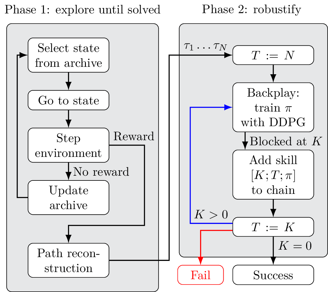
Fig. 1 describes PBCS. The algorithm is split in two successive phases, mirroring the Go-Explore framework. In a first phase, the environment is incrementally explored until a single rewarded state is found. In a second phase, a single trajectory provides a list of starting points, that are used to train DDPG on increasingly difficult portions of the full environment. Each time the problem becomes too difficult and DDPG starts to fail, training stops, and the trained agent is recorded as a local skill. Training then resumes for the next skill, with a new target state. This loop generates a set of skills that can then be chained together to create a controller that reaches the target reliably.
Notations
State neighborhood. For any state \(s\in S\), and \(\epsilon >0\), we define \(B_\epsilon (s)\) as the closed ball of radius \(\epsilon \) centered around \(s\). Formally, this is the set \(\left \{s’\in S\mid d(s,s’)\leq \epsilon \right \}\) where \(d\) is the L2 distance.
Skill chaining. Skill chaining consists in splitting a complex task into simpler sub-tasks that are each governed by a different policy. Complex tasks can then be solved by executing each policy sequentially.
Formally, each task \(T_i\) has an activation condition \(A_i~\subset ~S\), and a policy \(\pi _i: S\rightarrow A\). A task chain is a list of tasks \(T_0 \ldots T_n\), which can be executed sequentially: the actor uses \(\pi _0\) until the state of the system reaches a state \(s\in A_1\), then it uses \(\pi _1\), and so on until the end of the episode (which can be triggered by reaching either a terminal state or a predetermined maximum number of steps).
3.1 Phase 1: Explore until Solved
In phase 1, PBCS explores to find a single path that obtains a non-zero reward in the environment. This exploration phase is summarized in this section, and implementation details are available in Appendix S1. An archive keeps track of all the visited states. In this archive, states \(s\) are grouped in square state-space bins. A state-counter \(c_s\) is attached to each state, and a bin-counter \(c_b\) is attached to each bin. All counters are initialized to \(0\). :
- Select state from archive. To select a state, the non-empty bin with the lowest counter is first selected, then from all the states in this bin, the state with the lowest counter is selected. Both the bin and state counters are then incremented.
- Go to state. The environment is reset to the selected state. This assumes the existence of a “reset-anywhere” primitive, which can be made available in simulated environments.
- Step environment. A single environment step is performed, with a random action.
- Update archive. The newly-reached state is added to the archive if not already present.
- Termination of phase 1. As soon as the reward is reached, the archive is used to reconstruct the sequence of states that led the agent from its initial state to the reward. This sequence \(\tau _0 \ldots \tau _N\) is passed on to phase 2.
This process can be seen as a random walk with a constraint on the maximum distance between two states: in the beginning, a single trajectory is explored until it reaches a state that is too close to an already-visited state. When this happens, a random visited state is selected as the starting point of a new random walk. Another interpretation of this process is the construction of a set of states with uniform spatial density. Under this view, the number of states in each cell is used as a proxy for the spatial density of the distribution.
3.2 Phase 2: Robustify
Phase 2 of PBCS learns a controller from the trajectory obtained in phase 1.
Output: \(\pi _0\ldots \pi _n\) a chain of policies with activation sets \(A_0\ldots A_n\)
\(T = N\)
\(n = 0\)
while \(T>0\) do
\(\pi _n,T = \text{Backplay} (\tau _0\ldots \tau _T)\)
\(A_n = B_\epsilon (\tau _T)\)
\(n = n + 1\)
end
Reverse lists \(\pi _0\ldots \pi _n\) and \(A_0\ldots A_n\)
Skill Chaining
Algorithm 1 presents the skill chaining process. It uses the Backplay function, that takes as input a trajectory \(\tau _0\ldots \tau _T\), and returns a policy \(\pi \) and an index \(K<T\) such that running policy \(\pi \) repeatedly on a state from \(B_\epsilon (\tau _K)\) always leads to a state in \(B_\epsilon (\tau _T)\). The main loop builds a chain of skills that roughly follows trajectory \(\tau \), but is able to improve upon it. Specifically, activation sets \(A_n\) are centered around points of \(\tau \) but policies \(\pi _n\) are constructed using a generic RL algorithm that optimizes the path between two activation sets. The list of skills is then reversed, because it was constructed backwards.
Backplay.
The Backplay algorithm was originally proposed in [35]. More details on the differences between this original algorithm and our variant are available in section 1 and appendices. The Backplay function (Algorithm 2) takes as input a section \(\tau _0 \ldots \tau _T\) of the trajectory obtained in phase 1, and returns a \((K,\pi )\) pair where \(K\) is an index on trajectory \(\tau \), and \(\pi \) is a policy trained to reliably attain \(B_\epsilon (\tau _T)\) from \(B_\epsilon (\tau _K)\). The policy \(\pi \) is trained using DDPG to reach \(B_\epsilon (\tau _T)\) from starting point \(B_\epsilon (\tau _K)\), where \(K\) is initialized to \(T-1\), and gradually decremented in the main loop.
At each iteration, the algorithm evaluates the feasibility of a skill with target \(B_\epsilon (\tau _T)\), policy \(\pi \) and activation set \(B_\epsilon (\tau _K)\). If the measured performance is \(100\%\) without any training, the current skill is saved and the starting point is decremented. Otherwise, a training loop is executed until performance stabilizes (repeatedly until no improvement over the maximum performance is observed \(\alpha \) times in a row. We ran our experiments with \(\alpha =10\) , and a more in-depth discussion of hyperparameters is available in Appendix S2), and three cases are handled:
- The skill is always successful. The current skill is saved and the index of the starting point is decremented.
- The skill is never successful. The last successful skill is returned.
- The skill is sometimes successful. The current skill is not saved, and the index of the starting point is decremented. In our maze environment, this happens when \(B_\epsilon (\tau _K)\) overlaps a wall: in this case some states of \(B_\epsilon (\tau _K)\) cannot reach the target no matter the policy.
Output: \(\pi _s\) a trained policy, \(K_s\) the index of the starting point of the policy
\(K = T – 1\)
Initialize a DDPG architecture with policy \(\pi \)
while \(K>0\) do
Test performance of \(\pi \) between \(B_\epsilon (\tau _K)\) and \(B_\epsilon (\tau _T)\) over \(\beta \) episodes
if performance \(= 100\%\) then
\(\pi _s = \pi \), \(K_s = K\)
else
Run Train (Algorithm 3) repeatedly until performance stabilizes.
Test performance of \(\pi \) between \(B_\epsilon (\tau _K)\) and \(B_\epsilon (\tau _T)\) over \(\beta \) episodes
if performance \(= 100\%\) then
\(\pi _s = \pi \), \(K_s = K\)
end
if performance \(= 0\%\) and \(K_s\) exists then
return \((K_s, \pi _s)\)
end
end
\(K = K – 1\)
end
return \((K_s, \pi _s)\)
Reward Shaping.
With reward shaping, we bypass the reward function of the environment, and train DDPG to reach any state \(\tau _T\). We chose to use the method proposed by [28]: we define a potential function in Equation \eqref{eq:1a} where \(d(s,A_i)\) is the L2 distance between \(s\) and the center of \(A_i\). We then define our shaped reward in Equation \eqref{eq:1b}.
$$ \begin {equation} \Phi (s) = \frac {1}{d(s, A_i)} \tag{1a}\label{eq:1a}\end{equation}$$
$$ \begin {equation}R_\text {shaped}(s,a,s’) = \begin {cases}10&\text {if } s\in A_i \\ \Phi (s’) – \Phi (s)&\text {otherwise.}\end {cases} \tag{1b}\label{eq:1b}\end{equation}$$
Output: The average performance \(p\)
n = 0
for \(i=1\ldots \beta \) do
\(s \sim B_\epsilon (\tau _K)\)
for \(j=1\ldots \text {max\_steps}\) do
\(a = \pi (s) + \text {random noise}\)
\(s’ = \text {step}(s,a)\)
\(r = \begin {cases} 10&d(s’,\tau _T)\leq \epsilon \\ \frac {1}{d(s’,\tau _T)} – \frac {1}{d(s,\tau _T)}&\text {otherwise} \end {cases}\)
DDPG.train\((s,a,s’,r)\)
\(s = s’\)
if \(d(s’,\tau _T) \leq \epsilon \) then
n = n + 1
break
end
end
end
\(p=\frac {n}{\beta }\)
Algorithm 3 shows how this reward function is used in place of the environment reward. This training function runs \(\beta \) episodes of up to max_steps steps each, and returns the fraction of episodes that were able to reach the reward. \(\beta \) is a hyperparameter that we set to 50 for our test, and more details on this choice are available in Appendix S2 .
Importantly, reaching a performance of 100% is not always possible, even with long training sessions, because the starting point is selected in \(B_\epsilon (\tau _K)\), and some of these states may be inside obstacles for instance.
4 Experimental Results
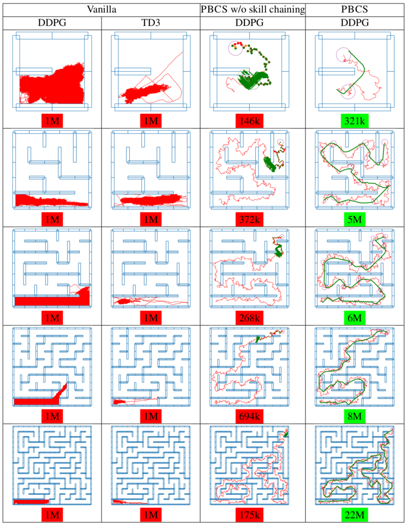
In ”Vanilla” experiments, the red paths represent the whole area explored by the RL algorithm. In ”Backplay” experiments, the trajectory computed in phase 1 is displayed in red, and the ”robustified” policy or policy chain is displayed in green. Activation sets \(A_i\) are displayed as purple circles. Enlarged images are presented in Fig. S2.
We perform experiments in continuous maze environments of various sizes. For a maze of size \(N\), the state-space is the position of a point mass in \([0,N]^2\) and the action describes the speed of the point mass, in \([-0.1, 0.1]^2\). Therefore, the step function is simply \(s’=s+a\), unless the \([s,s’]\) segment intersects a wall. The only reward is \(-1\) when hitting a wall and \(1\) when the target area is reached. A more formal definition of the environment is available in Appendix S4. . We first tested standard RL algorithms (DDPG and TD3), then PBCS, but without skill chaining (this was done by replacing the blue branch with the red branch in Fig. 1). When the full algorithm would add a new skill to the skill chain and continue training, this variant stops and fails. These results are presented in column ”PBCS without skill chaining”. Finally, the full version of PBCS with skill chaining is able to solve complex mazes up to \(15 \times 15\) cells, by chaining several intermediate skills.
5 Discussion of Results
As expected, standard RL algorithms (DDPG and TD3) were unable to solve all but the simplest mazes. These algorithms have no mechanism for state-space exploration other than uniform noise added to their policies during rollouts. Therefore, in the best-case scenario they perform a random walk and, in the worst-case scenario, their actors may actively hinder exploration.
More surprisingly, PBCS without skill chaining is still unable to reliably 2 solve mazes larger than \(2 \times 2\). Although phase 1 always succeeds in finding a feasible trajectory \(\tau \), the robustification phase fails relatively early. We attribute these failures to well-known limitations of DDPG exposed in Sect. 2. We found that the success rate of PBCS without skill chaining was very dependent on the discount rate \(\gamma \), which we discuss in Appendix S3.
The full version of PBCS with skill chaining is able to overcome these issues by limiting the length of training sessions of DDPG, and is able to solve complex mazes up to \(7 \times 7\), by chaining several intermediate skills.
6 Conclusion
The authors of Go-Explore identified state-space exploration as a fundamental difficulty on two Atari benchmarks. We believe that this difficulty is also present in many continuous control problems, especially in high-dimension environments. We have shown that the PBCS algorithm can solve these hard exploration, continuous control environments by combining a motion planning process with reinforcement learning and skill chaining. Further developments should focus on testing these hybrid approaches on higher dimensional environments that present difficult exploration challenges together with difficult local control, such as the Ant-Maze MuJoCo benchmark [44], and developing methods that use heuristics suited to continuous control in the exploration process, such as Quality-Diversity approaches [34].
References
1. Achiam, J., Knight, E., Abbeel, P.: Towards Characterizing Divergence in Deep Q-Learning. arXiv:1903.08894 (2019)
2. Benureau, F.C.Y., Oudeyer, P.Y.: Behavioral Diversity Generation in Autonomous Exploration through Reuse of Past Experience. Front. Robot. AI 3 (2016)
3. Burda, Y., Edwards, H., Storkey, A., Klimov, O.: Exploration by Random Network Distillation. arXiv:1810.12894 (2018)
4. Chiang, H.T.L., Hsu, J., Fiser, M., Tapia, L., Faust, A.: RL-RRT: Kinodynamic Motion Planning via Learning Reachability Estimators from RL Policies. arXiv:1907.04799 (2019)
5. Ciosek, K., Vuong, Q., Loftin, R., Hofmann, K.: Better Exploration with Optimistic Actor-Critic. arXiv:1910.12807 (2019)
6. Colas, C., Sigaud, O., Oudeyer, P.Y.: GEP-PG: Decoupling Exploration and Exploitation in Deep Reinforcement Learning Algorithms. arXiv:1802.05054 (2018)
7. Cully, A., Demiris, Y.: Quality and Diversity Optimization: A Unifying Modular Framework. IEEE Transactions on Evolutionary Computation 22 (2017)
8. Ecoffet, A., Huizinga, J., Lehman, J., Stanley, K.O., Clune, J.: Go-Explore: a New Approach for Hard-Exploration Problems. arXiv:1901.10995 (2019)
9. Erickson, L.H., LaValle, S.M.: Survivability: Measuring and ensuring path diversity. In: 2009 IEEE International Conference on Robotics and Automation. pp. 2068–2073 (2009)
10. Eysenbach, B., Gupta, A., Ibarz, J., Levine, S.: Diversity is All You Need: Learning Skills without a Reward Function. arXiv:1802.06070 (2018)
11. Faust, A., Ramirez, O., Fiser, M., Oslund, K., Francis, A., Davidson, J., Tapia, L.: PRM-RL: Long-range Robotic Navigation Tasks by Combining Reinforcement Learning and Sampling-based Planning. arXiv:1710.03937 (2018)
12. Florensa, C., Held, D., Wulfmeier, M., Zhang, M., Abbeel, P.: Reverse Curriculum Generation for Reinforcement Learning. arXiv:1707.05300 (2018)
13. Fournier, P., Sigaud, O., Colas, C., Chetouani, M.: CLIC: Curriculum Learning and Imitation for object Control in non-rewarding environments. arXiv:1901.09720 (2019)
14. Fujimoto, S., Hoof, H.v., Meger, D.: Addressing Function Approximation Error in Actor-Critic Methods. ICML (2018)
15. Fujimoto, S., Meger, D., Precup, D.: Off-Policy Deep Reinforcement Learning without Exploration. arXiv:1812.02900 (2018)
16. Goyal, A., Brakel, P., Fedus, W., Singhal, S., Lillicrap, T., Levine, S., Larochelle, H., Bengio, Y.: Recall Traces: Backtracking Models for Efficient Reinforcement Learning. arXiv:1804.00379 (2019)
17. van Hasselt, H., Doron, Y., Strub, F., Hessel, M., Sonnerat, N., Modayil, J.: Deep Reinforcement Learning and the Deadly Triad. arXiv:1812.02648 (2018)
18. Hosu, I.A., Rebedea, T.: Playing Atari Games with Deep Reinforcement Learning and Human Checkpoint Replay. arXiv:1607.05077 (2016)
19. Knepper, R.A., Mason, M.T.: Path diversity is only part of the problem. In: 2009 IEEE International Conference on Robotics and Automation. pp. 3224–3229 (2009)
20. Konidaris, G., Barto, A.G.: Skill Discovery in Continuous Reinforcement Learning Domains using Skill Chaining. In: Bengio, Y., et. al. (eds.) Advances in Neural Information Processing Systems 22, pp. 1015–1023 (2009)
21. Konidaris, G., Kuindersma, S., Grupen, R., Barto, A.G.: Constructing Skill Trees for Reinforcement Learning Agents from Demonstration Trajectories. In: Lafferty, J.D., et. al. (eds.) Advances in Neural Information Processing Systems 23, pp. 1162–1170 (2010)
22. Lavalle, S.M.: Rapidly-Exploring Random Trees: A New Tool for Path Planning. Tech. rep., Iowa State University (1998)
23. Lillicrap, T.P., Hunt, J.J., Pritzel, A., Heess, N., Erez, T., Tassa, Y., Silver, D., Wierstra, D.: Continuous control with deep reinforcement learning. arXiv:1509.02971 (2015)
24. Matheron, G., Perrin, N., Sigaud, O.: The problem with DDPG: understanding failures in deterministic environments with sparse rewards. arXiv:1911.11679 (2019)
25. Mnih, V., Kavukcuoglu, K., Silver, D., Graves, A., Antonoglou, I., Wierstra, D., Riedmiller, M.: Playing Atari with Deep Reinforcement Learning. arXiv:1312.5602 (2013)
26. Morere, P., Francis, G., Blau, T., Ramos, F.: Reinforcement Learning with Probabilistically Complete Exploration. arXiv:2001.06940 (2020)
27. Nair, A., McGrew, B., Andrychowicz, M., Zaremba, W., Abbeel, P.: Overcoming Exploration in Reinforcement Learning with Demonstrations. arXiv:1709.10089 (2018)
28. Ng, A.Y., Harada, D., Russell, S.J.: Policy Invariance Under Reward Transformations: Theory and Application to Reward Shaping. In: Proceedings of the Sixteenth International Conference on Machine Learning. pp. 278–287. ICML ’99 (1999)
29. Osband, I., Blundell, C., Pritzel, A., Van Roy, B.: Deep Exploration via Bootstrapped DQN. arXiv:1602.04621 (2016)
30. Paine, T.L., Gulcehre, C., Shahriari, B., Denil, M., Hoffman, M., Soyer, H., Tanburn, R., Kapturowski, S., Rabinowitz, N., Williams, D., Barth-Maron, G., Wang, Z., de Freitas, N.: Making Efficient Use of Demonstrations to Solve Hard Exploration Problems. arXiv:1909.01387 (2019)
31. Pathak, D., Agrawal, P., Efros, A.A., Darrell, T.: Curiosity-driven Exploration by Self-supervised Prediction. arXiv:1705.05363 (2017)
32. Penedones, H., Vincent, D., Maennel, H., Gelly, S., Mann, T., Barreto, A.: Temporal Difference Learning with Neural Networks – Study of the Leakage Propagation Problem. arXiv:1807.03064 (2018)
33. Pugh, J.K., Soros, L.B., Szerlip, P.A., Stanley, K.O.: Confronting the Challenge of Quality Diversity. In: Proceedings of the 2015 Annual Conference on Genetic and Evolutionary Computation. pp. 967–974. GECCO ’15, ACM, New York, NY, USA (2015)
34. Pugh, J.K., Soros, L.B., Stanley, K.O.: Quality Diversity: A New Frontier for Evolutionary Computation. Front. Robot. AI 3 (2016)
35. Resnick, C., Raileanu, R., Kapoor, S., Peysakhovich, A., Cho, K., Bruna, J.: Backplay: ”Man muss immer umkehren”. arXiv:1807.06919 (2018)
36. Riedmiller, M., Hafner, R., Lampe, T., Neunert, M., Degrave, J., Van de Wiele, T., Mnih, V., Heess, N., Springenberg, J.T.: Learning by Playing – Solving Sparse Reward Tasks from Scratch. arXiv:1802.10567 (2018)
37. Salimans, T., Chen, R.: Learning Montezuma’s Revenge from a Single Demonstration. arXiv:1812.03381 (2018)
38. Schaul, T., Quan, J., Antonoglou, I., Silver, D.: Prioritized Experience Replay. arXiv:1511.05952 (2015)
39. Schulman, J., Levine, S., Moritz, P., Jordan, M.I., Abbeel, P.: Trust Region Policy Optimization. arXiv:1502.05477 (2015)
40. Schulman, J., Wolski, F., Dhariwal, P., Radford, A., Klimov, O.: Proximal Policy Optimization Algorithms. arXiv:1707.06347 (2017)
41. Stadie, B.C., Levine, S., Abbeel, P.: Incentivizing Exploration In Reinforcement Learning With Deep Predictive Models. arXiv:1507.00814 (2015)
42. Sutton, R.S., Barto, A.G.: Reinforcement Learning: An Introduction. MIT Press (2018)
43. Tang, H., Houthooft, R., Foote, D., Stooke, A., Chen, X., Duan, Y., Schulman, J., De Turck, F., Abbeel, P.: #Exploration: A Study of Count-Based Exploration for Deep Reinforcement Learning. arXiv:1611.04717 (2016)
44. Tassa, Y., et. al.: DeepMind Control Suite. arXiv:1801.00690 (2018)
45. Wilson, E.B.: Probable Inference, the Law of Succession, and Statistical Inference. Journal of the American Statistical Association 22(158), 209–212 (1927)